Figure 1 shows the time-averaged energy distribution
function  , for different time periods and number of sheets. In
all figures, the thin solid curve is the energy distribution of the
isothermal distribution function of equation (3). What
we see is quite clear. As we make the time interval longer, the
time-averaged distribution function approaches to the isothermal
distribution. Thus, the numerical result suggests the system is
ergodic. However, it also shows that the time needed to populate the
high-energy region is very long. The sampling time interval is 128
time units for N=16, and 512 time units for N=64 and 128. Thus, in
the case of
, for different time periods and number of sheets. In
all figures, the thin solid curve is the energy distribution of the
isothermal distribution function of equation (3). What
we see is quite clear. As we make the time interval longer, the
time-averaged distribution function approaches to the isothermal
distribution. Thus, the numerical result suggests the system is
ergodic. However, it also shows that the time needed to populate the
high-energy region is very long. The sampling time interval is 128
time units for N=16, and 512 time units for N=64 and 128. Thus, in
the case of  and N=16 (dash-dotted curve in figure 1a), total
number of sample points is
and N=16 (dash-dotted curve in figure 1a), total
number of sample points is  .
.
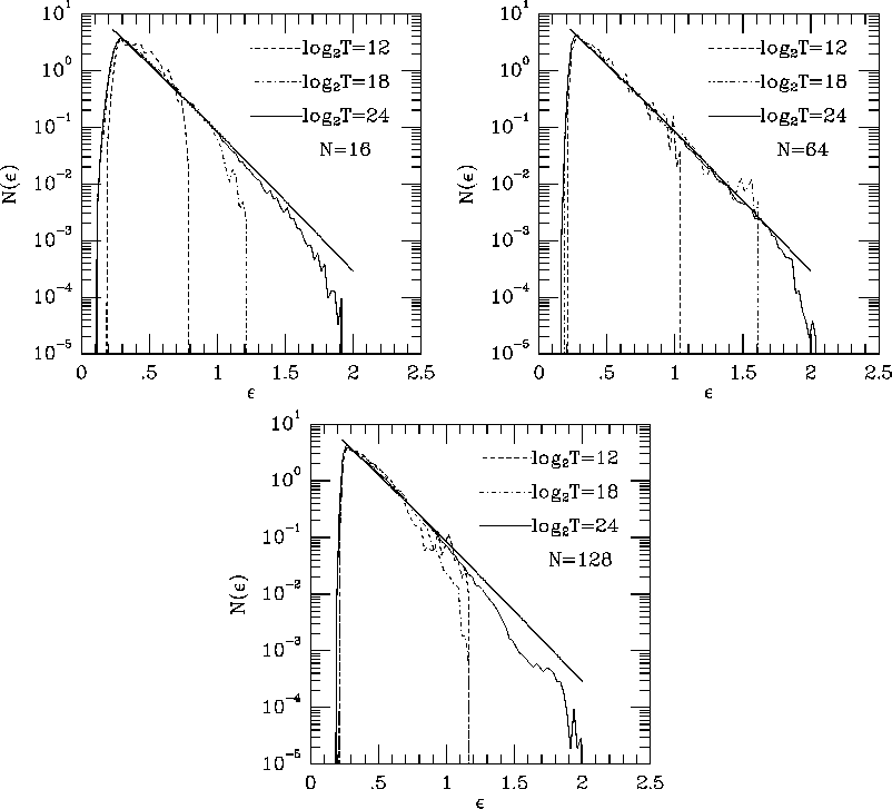
Figure 1: The time-averaged distribution function in the energy space
 ; (a) N=16, (b) N=64, (c) N=128.
If we can assume that the sample points are uncorrelated, the
possibility that no sample exceeds energy level  is
given simply by
is
given simply by

where

and n is the number of sample points. Figure 2 shows
 as a function of
  . For
. For
 ,
,  , and therefore the
probability that none of 32768 samples does not exceed
, and therefore the
probability that none of 32768 samples does not exceed  is practically zero (
 ). In other words, the numerical
result seems to suggest that the system is not in the thermally
relaxed state even after
). In other words, the numerical
result seems to suggest that the system is not in the thermally
relaxed state even after  crossing times.
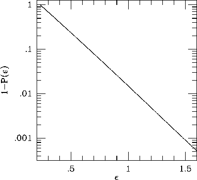
Figure 2: The compliment of the cumulative distribution function
 for the thermal equilibrium.
Of course, this result is not surprising if the relaxation time is
long. Samples taken with the time interval shorter than the
relaxation time have a strong correlation, and therefore the effective
number of freedom can be smaller than n. Roughly speaking, if the
relaxation time is longer than  , our numerical result is
consistent with the assumption that the system is in the thermal
equilibrium. In the next subsection, we investigate the relaxation
time itself.
, our numerical result is
consistent with the assumption that the system is in the thermal
equilibrium. In the next subsection, we investigate the relaxation
time itself.
We measured the following quantities:
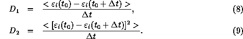
These quantities correspond to the coefficients of the first and second-order terms in the Fokker-Planck equation for the distribution function, and have been used as the measure of the relaxation in many studies (see, e.g., Hernquist and Barnes,[1] Hernquist et al. [2]), for three-dimensional systems. However, to our knowledge this measure has not been used for the study of the sheet model.
In order to see the dependence of these diffusion coefficients on the
energy, we calculated them for intervals of  . Figure
3 shows the results, for N=16, 64 and 256. The time
interval
. Figure
3 shows the results, for N=16, 64 and 256. The time
interval  was taken equal to
  . We used smaller values
for
. We used smaller values
for  and confirmed that the choice of
  has
negligible effect if
has
negligible effect if  is larger than
  and smaller
than
and smaller
than  . Time average is taken over the whole simulation period.
We can see that both the first- and second-order terms show very
strong dependence on the energy of the sheets, and of the order of
. Time average is taken over the whole simulation period.
We can see that both the first- and second-order terms show very
strong dependence on the energy of the sheets, and of the order of
 for
for  . Figure 3 suggests that the
relaxation timescale grows exponentially as energy grows. This
behavior is independent of the value of N.
. Figure 3 suggests that the
relaxation timescale grows exponentially as energy grows. This
behavior is independent of the value of N.
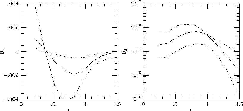
Figure 3: The diffusion coefficients (a)  and (b)
  plotted against
the energy e for three values of N. Long-dashed, solid, and
short-dashed curves are the results for N=16, 64 and 256, respectively.
plotted against
the energy e for three values of N. Long-dashed, solid, and
short-dashed curves are the results for N=16, 64 and 256, respectively.
We can define the relaxation timescale as

that is, the timescale in which energy changes significantly. Figure 4
shows this relaxation timescale for different values of N and  .
The relaxation time shows very strong
dependence on the energy and the relaxation of high-energy sheets is
much slower than that of sheets in lower energies. This is
partly because of the dependence of
.
The relaxation time shows very strong
dependence on the energy and the relaxation of high-energy sheets is
much slower than that of sheets in lower energies. This is
partly because of the dependence of  on
on  itself. However, as w
can see in figure 3, the dependence of the diffusion
coefficient is the main reason.
itself. However, as w
can see in figure 3, the dependence of the diffusion
coefficient is the main reason.
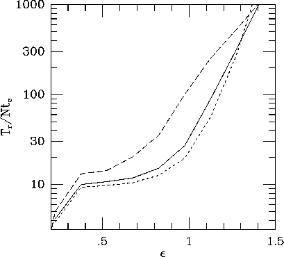
Figure 4: The relaxation time in unit of  plotted against
the energy e for three values of N. Curves have the same meanings
as in figure 3
plotted against
the energy e for three values of N. Curves have the same meanings
as in figure 3
This
result resolves the apparent contradiction between the fact that the
relaxation timescale is of the order of  [5] and
that the system reaches the true thermal equilibrium only in much
longer timescale.[12] It is true that the relaxation
timescale is
[5] and
that the system reaches the true thermal equilibrium only in much
longer timescale.[12] It is true that the relaxation
timescale is  , but the coefficient before N is quite large, in
particular for sheets with high energies.
, but the coefficient before N is quite large, in
particular for sheets with high energies.
An important question is why the relaxation timescale depends so strongly on the energy. This is provably due to the fact that high-energy sheets have the orbital period significantly longer than the crossing time. Typical sheets have the period comparable to the crossing time, and therefore they are in strong resonance with each other. However, a high-energy sheet has the period longer than the crossing time, and thus it is out of resonance with the rest of the system. Therefore, the coupling between high energy sheets and the rest of the system is much weaker than the coupling between sheets with average energy. This explains why the relaxation of high energy sheets is slow.