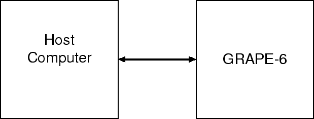
GRAPE-6 is the successor of GRAPE-4, designed for high-accuracy integration of gravitational N-body system using the individual timestep and Hermite scheme. It works as a backend processor, connected to a host computer through PCI interface. Thus, from the viewpoint of a user, GRAPE-6 system (single cluster) looks like that in figure 1.
In the following, I first describe what is calculated how, first on this simple (single cluster, or SC) configuration. What GRAPE-6 SC calculates is the forces and their time derivative on 48 particles, from all particles loaded into its memory.
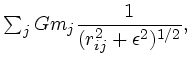
To be more precise, GRAPE-6 calculates the following
| (4) | |||
| (5) |
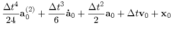
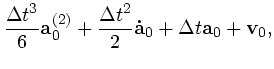
The position and velocity of particle ![]() have additional suffix
have additional suffix ![]() to denote they are ``predicted'' values at time
to denote they are ``predicted'' values at time ![]() using the
following formulae:
using the
following formulae:
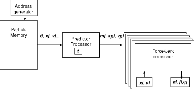
Thus, from the viewpoint of the host computer (and the application program on the host), the internal structure of GRAPE-6 SC looks like that in figure 2.
If you have multiple clusters connected to a single host, they work just completely independently. In all library functions that actually communicate with GRAPE-6 hardware, you simply specify the identity of the cluster as an argument.
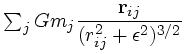
![$\textstyle \sum_jGm_j\left[
\displaystyle{{\bf v}_{ij} \over (r_{ij}^2+\epsilon...
...{ij}\cdot {\bf r}_{ij}) {\bf r}_{ij} \over
(r_{ij}^2+\epsilon^2)^{5/2}}\right],$](img5.png)